

Recurrent Neural Networks (RNN) are widely used for modelling sequential data, such as music and sentences. In this example, we use SINGA to train a RNN model proposed by Tomas Mikolov for language modeling. The training objective (loss) is to minimize the perplexity per word, which is equivalent to maximize the probability of predicting the next word given the current word in a sentence.
Different to the CNN, MLP and RBM examples which use built-in layers(layer) and records(data), none of the layers in this example are built-in. Hence users would learn to implement their own layers and data records through this example.
In SINGA_ROOT/examples/rnnlm/, scripts are provided to run the training job. First, the data is prepared by
$ cp Makefile.example Makefile
$ make download
$ make create
Second, to compile the source code under examples/rnnlm/, run
$ make rnnlm
An executable file rnnlm.bin will be generated.
Third, the training is started by passing rnnlm.bin and the job configuration to singa-run.sh,
# at SINGA_ROOT/
# export LD_LIBRARY_PATH=.libs:$LD_LIBRARY_PATH
$ ./bin/singa-run.sh -exec examples/rnnlm/rnnlm.bin -conf examples/rnnlm/job.conf
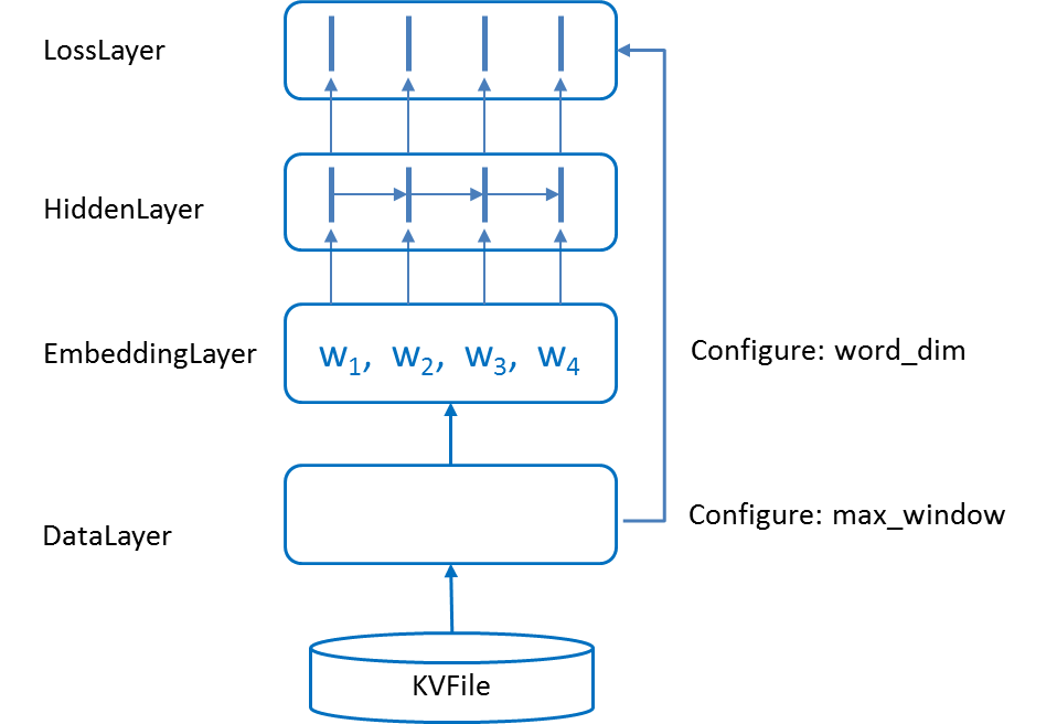 Figure 1 - Net structure of the RNN model.
The neural net structure is shown Figure 1. Word records are loaded by DataLayer. For every iteration, at most max_window word records are processed. If a sentence ending character is read, the DataLayer stops loading immediately. EmbeddingLayer looks up a word embedding matrix to extract feature vectors for words loaded by the DataLayer. These features are transformed by the HiddenLayer which propagates the features from left to right. The output feature for word at position k is influenced by words from position 0 to k-1. Finally, LossLayer computes the cross-entropy loss (see below) by predicting the next word of each word. The cross-entropy loss is computed as
$$L(w_t)=-log P(w_{t+1}|w_t)$$
Given $w_t$ the above equation would compute over all words in the vocabulary, which is time consuming. RNNLM Toolkit accelerates the computation as
$$P(w_{t+1}|w_t) = P(C_{w_{t+1}}|w_t) * P(w_{t+1}|C_{w_{t+1}})$$
Words from the vocabulary are partitioned into a user-defined number of classes. The first term on the left side predicts the class of the next word, and then predicts the next word given its class. Both the number of classes and the words from one class are much smaller than the vocabulary size. The probabilities can be calculated much faster.
The perplexity per word is computed by,
$$PPL = 10^{- avg_t log_{10} P(w_{t+1}|w_t)}$$
We use a small dataset provided by the RNNLM Toolkit. It has 10,000 training sentences, with 71350 words in total and 3720 unique words. The subsequent steps follow the instructions in Data Preparation to convert the raw data into records and insert them into data stores.
We define the word record as follows,
# in SINGA_ROOT/examples/rnnlm/rnnlm.proto
message WordRecord {
  optional string word = 1;
  optional int32 word_index = 2;
  optional int32 class_index = 3;
  optional int32 class_start = 4;
  optional int32 class_end = 5;
}
It includes the word string and its index in the vocabulary. Words in the vocabulary are sorted based on their frequency in the training dataset. The sorted list is cut into 100 sublists such that each sublist has 1/100 total word frequency. Each sublist is called a class. Hence each word has a class_index ([0,100)). The class_start is the index of the first word in the same class as word. The class_end is the index of the first word in the next class.
We use code from RNNLM Toolkit to read words, and sort them into classes. The main function in create_store.cc first creates word classes based on the training dataset. Second it calls the following function to create data store for the training, validation and test dataset.
int create_data(const char *input_file, const char *output_file);
input is the path to training/validation/testing text file from the RNNLM Toolkit, output is output store file. This function starts with
singa::io::KVFile store;
store.Open(output, signa::io::kCreate);
Then it reads the words one by one. For each word it creates a WordRecord instance, and inserts it into the store,
int wcnt = 0; // word count
WordRecord  wordRecord;
while(1) {
  readWord(wordstr, fin);
  if (feof(fin)) break;
  ...// fill in the wordRecord;
  string val;
  wordRecord.SerializeToString(&val);
  int length = snprintf(key, BUFFER_LEN, "%05d", wcnt++);
  store.Write(string(key, length), val);
}
Compilation and running commands are provided in the Makefile.example. After executing
make create
train_data.bin, test_data.bin and valid_data.bin will be created.
4 user-defined layers are implemented for this application. Following the guide for implementing new Layer subclasses, we extend the LayerProto to include the configuration messages of user-defined layers as shown below (3 out of the 7 layers have specific configurations),
import "job.proto";     // Layer message for SINGA is defined

//For implementation of RNNLM application
extend singa.LayerProto {
  optional EmbeddingProto embedding_conf = 101;
  optional LossProto loss_conf = 102;
  optional DataProto data_conf = 103;
}
In the subsequent sections, we describe the implementation of each layer, including its configuration message.
This is the base layer of all other layers for this applications. It is defined as follows,
class RNNLayer : virtual public Layer {
public:
  inline int window() { return window_; }
protected:
  int window_;
};
For this application, two iterations may process different number of words. Because sentences have different lengths. The DataLayer decides the effective window size. All other layers call its source layers to get the effective window size and resets window_ in ComputeFeature function.
DataLayer is for loading Records.
class DataLayer : public RNNLayer, singa::InputLayer {
 public:
  void Setup(const LayerProto& proto, const vector<Layer*>& srclayers) override;
  void ComputeFeature(int flag, const vector<Layer*>& srclayers) override;
  int max_window() const {
    return max_window_;
  }
 private:
  int max_window_;
  singa::io::Store* store_;
};
The Setup function gets the user configured max window size.
max_window_ = proto.GetExtension(input_conf).max_window();
The ComputeFeature function loads at most max_window records. It could also stop when the sentence ending character is encountered.
...// shift the last record to the first
window_ = max_window_;
for (int i = 1; i <= max_window_; i++) {
  // load record; break if it is the ending character
}
The configuration of DataLayer is like
name: "data"
user_type: "kData"
[data_conf] {
  path: "examples/rnnlm/train_data.bin"
  max_window: 10
}
This layer gets records from DataLayer. For each record, the word index is parsed and used to get the corresponding word feature vector from the embedding matrix.
The class is declared as follows,
class EmbeddingLayer : public RNNLayer {
  ...
  const std::vector<Param*> GetParams() const override {
    std::vector<Param*> params{embed_};
    return params;
  }
 private:
  int word_dim_, vocab_size_;
  Param* embed_;
}
The embed_ field is a matrix whose values are parameter to be learned. The matrix size is vocab_size_ x word_dim_.
The Setup function reads configurations for word_dim_ and vocab_size_. Then it allocates feature Blob for max_window words and setups embed_.
int max_window = srclayers[0]->data(this).shape()[0];
word_dim_ = proto.GetExtension(embedding_conf).word_dim();
data_.Reshape(vector<int>{max_window, word_dim_});
...
embed_->Setup(vector<int>{vocab_size_, word_dim_});
The ComputeFeature function simply copies the feature vector from the embed_ matrix into the feature Blob.
# reset effective window size
window_ = datalayer->window();
auto records = datalayer->records();
...
for (int t = 0; t < window_; t++) {
  int idx  <- word index
  Copy(words[t], embed[idx]);
}
The ComputeGradient function copies back the gradients to the embed_ matrix.
The configuration for EmbeddingLayer is like,
user_type: "kEmbedding"
[embedding_conf] {
  word_dim: 15
  vocab_size: 3720
}
srclayers: "data"
param {
  name: "w1"
  init {
    type: kUniform
    low:-0.3
    high:0.3
  }
}
This layer unrolls the recurrent connections for at most max_window times. The feature for position k is computed based on the feature from the embedding layer (position k) and the feature at position k-1 of this layer. The formula is
$$f[k]=\sigma (f[t-1]*W+src[t])$$
where $W$ is a matrix with word_dim_ x word_dim_ parameters.
If you want to implement a recurrent neural network following our design, this layer is of vital importance for you to refer to.
class HiddenLayer : public RNNLayer {
  ...
  const std::vector<Param*> GetParams() const override {
    std::vector<Param*> params{weight_};
    return params;
  }
private:
  Param* weight_;
};
The Setup function setups the weight matrix as
weight_->Setup(std::vector<int>{word_dim, word_dim});
The ComputeFeature function gets the effective window size (window_) from its source layer i.e., the embedding layer. Then it propagates the feature from position 0 to position window_ -1. The detailed descriptions for this process are illustrated as follows.
void HiddenLayer::ComputeFeature() {
  for(int t = 0; t < window_size; t++){
    if(t == 0)
      Copy(data[t], src[t]);
    else
      data[t]=sigmoid(data[t-1]*W + src[t]);
  }
}
The ComputeGradient function computes the gradient of the loss w.r.t. W and the source layer. Particularly, for each position k, since data[k] contributes to data[k+1] and the feature at position k in its destination layer (the loss layer), grad[k] should contains the gradient from two parts. The destination layer has already computed the gradient from the loss layer into grad[k]; In the ComputeGradient function, we need to add the gradient from position k+1.
void HiddenLayer::ComputeGradient(){
  ...
  for (int k = window_ - 1; k >= 0; k--) {
    if (k < window_ - 1) {
      grad[k] += dot(grad[k + 1], weight.T()); // add gradient from position t+1.
    }
    grad[k] =... // compute gL/gy[t], y[t]=data[t-1]*W+src[t]
  }
  gweight = dot(data.Slice(0, window_-1).T(), grad.Slice(1, window_));
  Copy(gsrc, grad);
}
After the loop, we get the gradient of the loss w.r.t y[k], which is used to compute the gradient of W and the src[k].
This layer computes the cross-entropy loss and the $log_{10}P(w_{t+1}|w_t)$ (which could be averaged over all words by users to get the PPL value).
There are two configuration fields to be specified by users.
message LossProto {
  optional int32 nclass = 1;
  optional int32 vocab_size = 2;
}
There are two weight matrices to be learned
class LossLayer : public RNNLayer {
  ...
 private:
  Param* word_weight_, *class_weight_;
}
The ComputeFeature function computes the two probabilities respectively.
$$P(C_{w_{t+1}}|w_t) = Softmax(w_t * class\_weight_)$$ $$P(w_{t+1}|C_{w_{t+1}}) = Softmax(w_t * word\_weight[class\_start:class\_end])$$
$w_t$ is the feature from the hidden layer for the k-th word, its ground truth next word is $w_{t+1}$. The first equation computes the probability distribution over all classes for the next word. The second equation computes the probability distribution over the words in the ground truth class for the next word.
The ComputeGradient function computes the gradient of the source layer (i.e., the hidden layer) and the two weight matrices.
We employ kFixedStep type of the learning rate change method and the configuration is as follows. We decay the learning rate once the performance does not increase on the validation dataset.
updater{
  type: kSGD
  learning_rate {
    type: kFixedStep
    fixedstep_conf:{
      step:0
      step:48810
      step:56945
      step:65080
      step:73215
      step_lr:0.1
      step_lr:0.05
      step_lr:0.025
      step_lr:0.0125
      step_lr:0.00625
    }
  }
}