

This example uses SINGA to train 4 RBM models and one auto-encoder model over the MNIST dataset. The auto-encoder model is trained to reduce the dimensionality of the MNIST image feature. The RBM models are trained to initialize parameters of the auto-encoder model. This example application is from Hinton’s science paper.
Running scripts are provided in SINGA_ROOT/examples/rbm folder.
The MNIST dataset has 70,000 handwritten digit images. The data preparation page has details on converting this dataset into SINGA recognizable format. Users can simply run the following commands to download and convert the dataset.
# at SINGA_ROOT/examples/mnist/
$ cp Makefile.example Makefile
$ make download
$ make create
The training is separated into two phases, namely pre-training and fine-tuning. The pre-training phase trains 4 RBMs in sequence,
# at SINGA_ROOT/
$ ./bin/singa-run.sh -conf examples/rbm/rbm1.conf
$ ./bin/singa-run.sh -conf examples/rbm/rbm2.conf
$ ./bin/singa-run.sh -conf examples/rbm/rbm3.conf
$ ./bin/singa-run.sh -conf examples/rbm/rbm4.conf
The fine-tuning phase trains the auto-encoder by,
$ ./bin/singa-run.sh -conf examples/rbm/autoencoder.conf
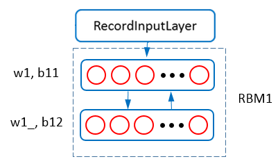 Figure 1 - RBM1.
The neural net structure for training RBM1 is shown in Figure 1. The data layer and parser layer provides features for training RBM1. The visible layer (connected with parser layer) of RBM1 accepts the image feature (784 dimension). The hidden layer is set to have 1000 neurons (units). These two layers are configured as,
layer{
  name: "RBMVis"
  type: kRBMVis
  srclayers:"mnist"
  srclayers:"RBMHid"
  rbm_conf{
    hdim: 1000
  }
  param{
    name: "w1"
    init{
      type: kGaussian
      mean: 0.0
      std: 0.1
    }
  }
  param{
    name: "b11"
    init{
      type: kConstant
      value: 0.0
    }
  }
}

layer{
  name: "RBMHid"
  type: kRBMHid
  srclayers:"RBMVis"
  rbm_conf{
    hdim: 1000
  }
  param{
    name: "w1_"
    share_from: "w1"
  }
  param{
    name: "b12"
    init{
      type: kConstant
      value: 0.0
    }
  }
}
For RBM, the weight matrix is shared by the visible and hidden layers. For instance, w1 is shared by vis and hid layers shown in Figure 1. In SINGA, we can configure the share_from field to enable parameter sharing as shown above for the param w1 and w1_.
Contrastive Divergence is configured as the algorithm for TrainOneBatch. Following Hinton’s paper, we configure the updating protocol as follows,
# Updater Configuration
updater{
  type: kSGD
  momentum: 0.2
  weight_decay: 0.0002
  learning_rate{
    base_lr: 0.1
    type: kFixed
  }
}
Since the parameters of RBM0 will be used to initialize the auto-encoder, we should configure the workspace field to specify a path for the checkpoint folder. For example, if we configure it as,
cluster {
  workspace: "examples/rbm/rbm1/"
}
Then SINGA will checkpoint the parameters into examples/rbm/rbm1/.
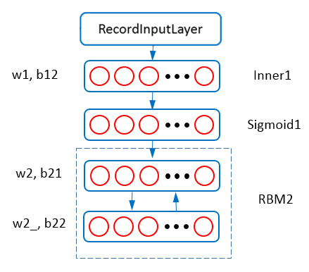 Figure 2 - RBM2.
Figure 2 shows the net structure of training RBM2. The visible units of RBM2 accept the output from the Sigmoid1 layer. The Inner1 layer is a InnerProductLayer whose parameters are set to the w1 and b12 learned from RBM1. The neural net configuration is (with layers for data layer and parser layer omitted).
layer{
  name: "Inner1"
  type: kInnerProduct
  srclayers:"mnist"
  innerproduct_conf{
    num_output: 1000
  }
  param{ name: "w1" }
  param{ name: "b12"}
}

layer{
  name: "Sigmoid1"
  type: kSigmoid
  srclayers:"Inner1"
}

layer{
  name: "RBMVis"
  type: kRBMVis
  srclayers:"Sigmoid1"
  srclayers:"RBMHid"
  rbm_conf{
    hdim: 500
  }
  param{
    name: "w2"
    ...
  }
  param{
    name: "b21"
    ...
  }
}

layer{
  name: "RBMHid"
  type: kRBMHid
  srclayers:"RBMVis"
  rbm_conf{
    hdim: 500
  }
  param{
    name: "w2_"
    share_from: "w2"
  }
  param{
    name: "b22"
    ...
  }
}
To load w0 and b02 from RBM0’s checkpoint file, we configure the checkpoint_path as,
checkpoint_path: "examples/rbm/rbm1/checkpoint/step6000-worker0"
cluster{
  workspace: "examples/rbm/rbm2"
}
The workspace is changed for checkpointing w2, b21 and b22 into examples/rbm/rbm2/.
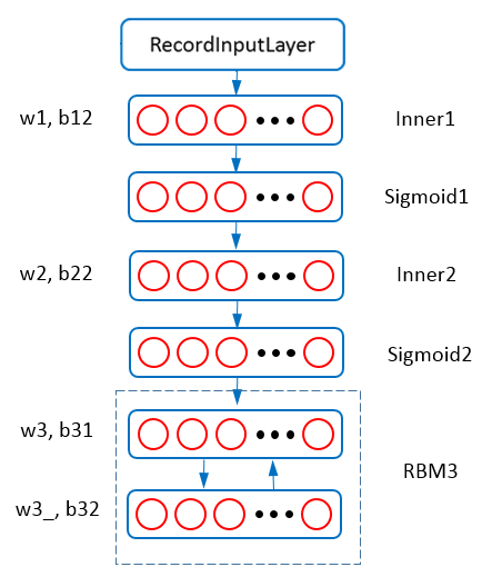 Figure 3 - RBM3.
Figure 3 shows the net structure of training RBM3. In this model, a layer with 250 units is added as the hidden layer of RBM3. The visible units of RBM3 accepts output from Sigmoid2 layer. Parameters of Inner1 and Innner2 are set to w1,b12,w2,b22 which can be load from the checkpoint file of RBM2, i.e., “examples/rbm/rbm2/”.
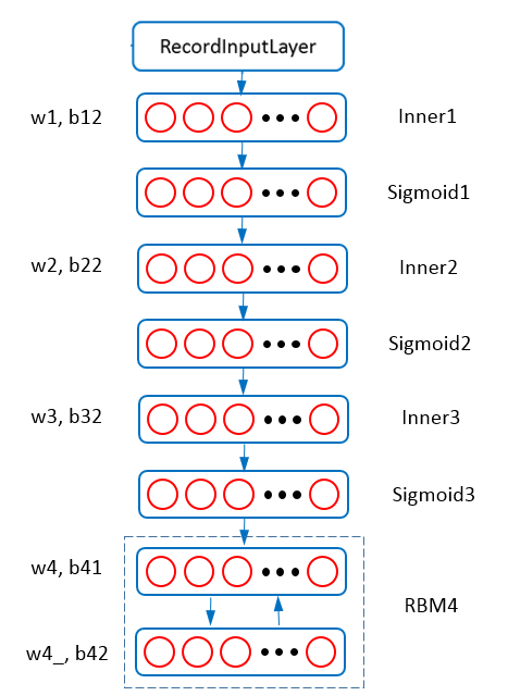 Figure 4 - RBM4.
Figure 4 shows the net structure of training RBM4. It is similar to Figure 3, but according to Hinton’s science paper, the hidden units of the top RBM (RBM4) have stochastic real-valued states drawn from a unit variance Gaussian whose mean is determined by the input from the RBM’s logistic visible units. So we add a gaussian field in the RBMHid layer to control the sampling distribution (Gaussian or Bernoulli). In addition, this RBM has a much smaller learning rate (0.001). The neural net configuration for the RBM4 and the updating protocol is (with layers for data layer and parser layer omitted),
# Updater Configuration
updater{
  type: kSGD
  momentum: 0.9
  weight_decay: 0.0002
  learning_rate{
    base_lr: 0.001
    type: kFixed
  }
}

layer{
  name: "RBMVis"
  type: kRBMVis
  srclayers:"Sigmoid3"
  srclayers:"RBMHid"
  rbm_conf{
    hdim: 30
  }
  param{
    name: "w4"
    ...
  }
  param{
    name: "b41"
    ...
  }
}

layer{
  name: "RBMHid"
  type: kRBMHid
  srclayers:"RBMVis"
  rbm_conf{
    hdim: 30
    gaussian: true
  }
  param{
    name: "w4_"
    share_from: "w4"
  }
  param{
    name: "b42"
    ...
  }
}
In the fine-tuning stage, the 4 RBMs are “unfolded” to form encoder and decoder networks that are initialized using the parameters from the previous 4 RBMs.
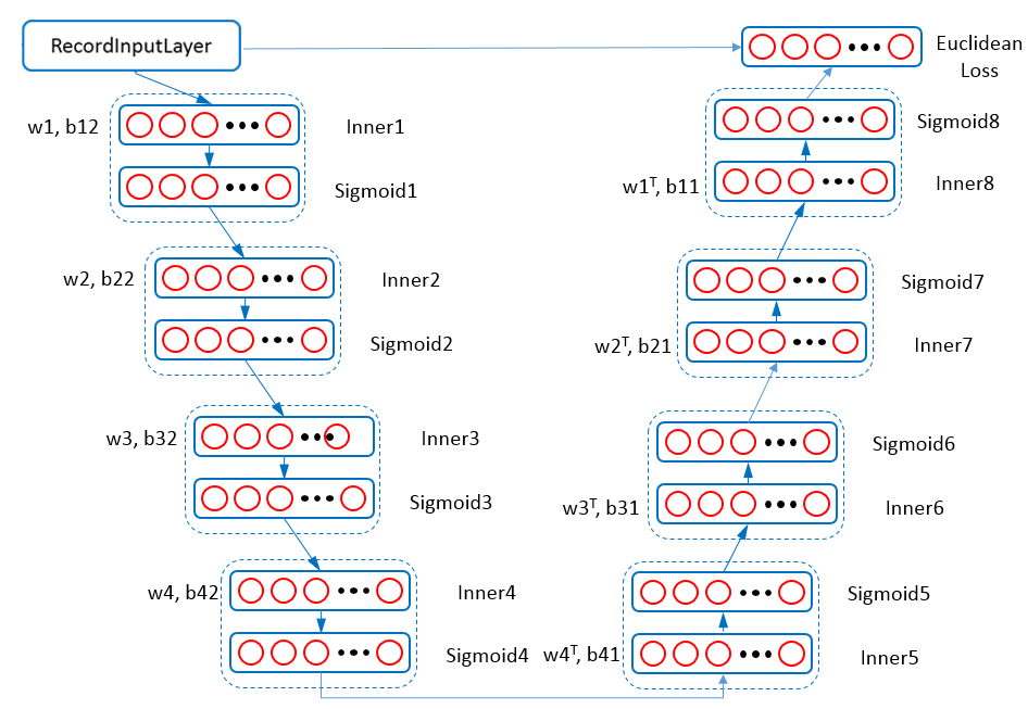 Figure 5 - Auto-Encoders.
Figure 5 shows the neural net structure for training the auto-encoder. Back propagation (kBP) is configured as the algorithm for TrainOneBatch. We use the same cluster configuration as RBM models. For updater, we use AdaGrad algorithm with fixed learning rate.
### Updater Configuration
updater{
  type: kAdaGrad
  learning_rate{
  base_lr: 0.01
  type: kFixed
  }
}
According to Hinton’s science paper, we configure a EuclideanLoss layer to compute the reconstruction error. The neural net configuration is (with some of the middle layers omitted),
layer{ name: "data" }
layer{ name:"mnist" }
layer{
  name: "Inner1"
  param{ name: "w1" }
  param{ name: "b12" }
}
layer{ name: "Sigmoid1" }
...
layer{
  name: "Inner8"
  innerproduct_conf{
    num_output: 784
    transpose: true
  }
  param{
    name: "w8"
    share_from: "w1"
  }
  param{ name: "b11" }
}
layer{ name: "Sigmoid8" }

# Euclidean Loss Layer Configuration
layer{
  name: "loss"
  type:kEuclideanLoss
  srclayers:"Sigmoid8"
  srclayers:"mnist"
}
To load pre-trained parameters from the 4 RBMs’ checkpoint file we configure checkpoint_path as
### Checkpoint Configuration
checkpoint_path: "examples/rbm/checkpoint/rbm1/checkpoint/step6000-worker0"
checkpoint_path: "examples/rbm/checkpoint/rbm2/checkpoint/step6000-worker0"
checkpoint_path: "examples/rbm/checkpoint/rbm3/checkpoint/step6000-worker0"
checkpoint_path: "examples/rbm/checkpoint/rbm4/checkpoint/step6000-worker0"
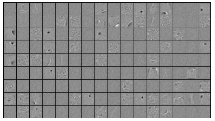
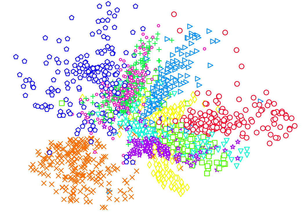
Figure 6 visualizes sample columns of the weight matrix of RBM1, We can see the Gabor-like filters are learned. Figure 7 depicts the features extracted from the top-layer of the auto-encoder, wherein one point represents one image. Different colors represent different digits. We can see that most images are well clustered according to the ground truth.