
NeuralNet in SINGA represents an instance of user’s neural net model. As the neural net typically consists of a set of layers, NeuralNet comprises a set of unidirectionally connected Layers. This page describes how to convert an user’s neural net into the configuration of NeuralNet.
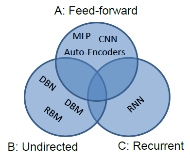 Figure 1 - Categorization of popular deep learning models.
Users configure the NeuralNet by listing all layers of the neural net and specifying each layer’s source layer names. Popular deep learning models can be categorized as Figure 1. The subsequent sections give details for each category.
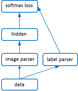 Figure 2 - Net structure of a MLP model.
Feed-forward models, e.g., CNN and MLP, can easily get configured as their layer connections are undirected without circles. The configuration for the MLP model shown in Figure 1 is as follows,
net {
  layer {
    name : 'data"
    type : kData
  }
  layer {
    name : 'image"
    type : kImage
    srclayer: 'data'
  }
  layer {
    name : 'label"
    type : kLabel
    srclayer: 'data'
  }
  layer {
    name : 'hidden"
    type : kHidden
    srclayer: 'image'
  }
  layer {
    name : 'softmax"
    type : kSoftmaxLoss
    srclayer: 'hidden'
    srclayer: 'label'
  }
}
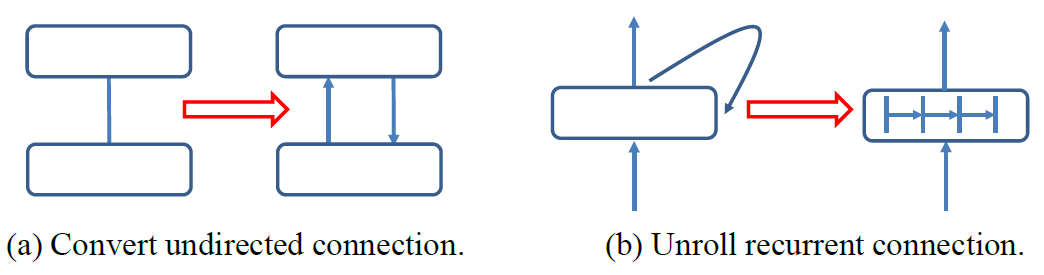 Figure 3 - Convert connections in RBM and RNN.
For energy models including RBM, DBM, etc., their connections are undirected (i.e., Category B). To represent these models using NeuralNet, users can simply replace each connection with two directed connections, as shown in Figure 3a. In other words, for each pair of connected layers, their source layer field should include each other’s name. The full RBM example has detailed neural net configuration for a RBM model, which looks like
net {
  layer {
    name : "vis"
    type : kVisLayer
    param {
      name : "w1"
    }
    srclayer: "hid"
  }
  layer {
    name : "hid"
    type : kHidLayer
    param {
      name : "w2"
      share_from: "w1"
    }
    srclayer: "vis"
  }
}
For recurrent neural networks (RNN), users can remove the recurrent connections by unrolling the recurrent layer. For example, in Figure 3b, the original layer is unrolled into a new layer with 4 internal layers. In this way, the model is like a normal feed-forward model, thus can be configured similarly. The RNN example has a full neural net configuration for a RNN model.
Typically, a training job includes three neural nets for training, validation and test phase respectively. The three neural nets share most layers except the data layer, loss layer or output layer, etc.. To avoid redundant configurations for the shared layers, users can uses the exclude filed to filter a layer in the neural net, e.g., the following layer will be filtered when creating the testing NeuralNet.
layer {
  ...
  exclude : kTest # filter this layer for creating test net
}
A neural net can be partitioned in different ways to distribute the training over multiple workers.
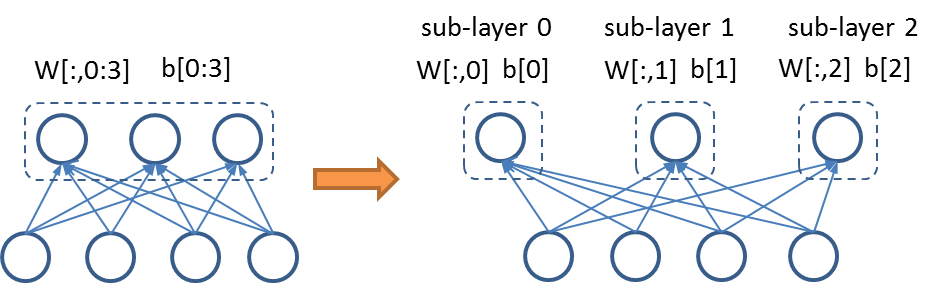 Figure 4 - Partitioning of a fully connected layer.
Every layer’s feature blob is considered a matrix whose rows are feature vectors. Thus, one layer can be split on two dimensions. Partitioning on dimension 0 (also called batch dimension) slices the feature matrix by rows. For instance, if the mini-batch size is 256 and the layer is partitioned into 2 sub-layers, each sub-layer would have 128 feature vectors in its feature blob. Partitioning on this dimension has no effect on the parameters, as every Param object is replicated in the sub-layers. Partitioning on dimension 1 (also called feature dimension) slices the feature matrix by columns. For example, suppose the original feature vector has 50 units, after partitioning into 2 sub-layers, each sub-layer would have 25 units. This partitioning may result in Param object being split, as shown in Figure 4. Both the bias vector and weight matrix are partitioned into two sub-layers.
There are 4 partitioning schemes, whose configurations are give below,
Partitioning each singe layer into sub-layers on batch dimension (see below). It is enabled by configuring the partition dimension of the layer to 0, e.g.,
  # with other fields omitted
  layer {
    partition_dim: 0
  }
Partitioning each singe layer into sub-layers on feature dimension (see below). It is enabled by configuring the partition dimension of the layer to 1, e.g.,
  # with other fields omitted
  layer {
    partition_dim: 1
  }
Partitioning all layers into different subsets. It is enabled by configuring the location ID of a layer, e.g.,
  # with other fields omitted
  layer {
    location: 1
  }
  layer {
    location: 0
  }
Hybrid partitioning of strategy 1, 2 and 3. The hybrid partitioning is useful for large models. An example application is to implement the idea proposed by Alex. Hybrid partitioning is configured like,
  # with other fields omitted
  layer {
    location: 1
  }
  layer {
    location: 0
  }
  layer {
    partition_dim: 0
    location: 0
  }
  layer {
    partition_dim: 1
    location: 0
  }
Currently SINGA supports strategy-2 well. Other partitioning strategies are are under test and will be released in later version.
Parameters can be shared in two cases,
sharing parameters among layers via user configuration. For example, the visible layer and hidden layer of a RBM shares the weight matrix, which is configured through the share_from field as shown in the above RBM configuration. The configurations must be the same (except name) for shared parameters.
due to neural net partitioning, some Param objects are replicated into different workers, e.g., partitioning one layer on batch dimension. These workers share parameter values. SINGA controls this kind of parameter sharing automatically, users do not need to do any configuration.
the NeuralNet for training and testing (and validation) share most layers , thus share Param values.
If the shared Param instances resident in the same process (may in different threads), they use the same chunk of memory space for their values. But they would have different memory spaces for their gradients. In fact, their gradients will be averaged by the stub or server.
static shared_ptr<NeuralNet> NeuralNet::Create(const NetProto& np, Phase phase, int num);
The above function creates a NeuralNet for a given phase, and returns a shared pointer to the NeuralNet instance. The phase is in {kTrain, kValidation, kTest}. num is used for net partitioning which indicates the number of partitions. Typically, a training job includes three neural nets for training, validation and test phase respectively. The three neural nets share most layers except the data layer, loss layer or output layer, etc.. The Create function takes in the full net configuration including layers for training, validation and test. It removes layers for phases other than the specified phase based on the exclude field in layer configuration:
layer {
  ...
  exclude : kTest # filter this layer for creating test net
}
The filtered net configuration is passed to the constructor of NeuralNet:
NeuralNet::NeuralNet(NetProto netproto, int npartitions);
The constructor creates a graph representing the net structure firstly in
Graph* NeuralNet::CreateGraph(const NetProto& netproto, int npartitions);
Next, it creates a layer for each node and connects layers if their nodes are connected.
void NeuralNet::CreateNetFromGraph(Graph* graph, int npartitions);
Since the NeuralNet instance may be shared among multiple workers, the Create function returns a shared pointer to the NeuralNet instance .
Param sharing is enabled by first sharing the Param configuration (in NeuralNet::Create) to create two similar (e.g., the same shape) Param objects, and then calling (in NeuralNet::CreateNetFromGraph),
void Param::ShareFrom(const Param& from);
It is also possible to share Params of two nets, e.g., sharing parameters of the training net and the test net,
void NeuralNet:ShareParamsFrom(shared_ptr<NeuralNet> other);
It will call Param::ShareFrom for each Param object.
NeuralNet provides a couple of access function to get the layers and params of the net:
const std::vector<Layer*>& layers() const;
const std::vector<Param*>& params() const ;
Layer* name2layer(string name) const;
Param* paramid2param(int id) const;
SINGA partitions the neural net in CreateGraph function, which creates one node for each (partitioned) layer. For example, if one layer’s partition dimension is 0 or 1, then it creates npartition nodes for it; if the partition dimension is -1, a single node is created, i.e., no partitioning. Each node is assigned a partition (or location) ID. If the original layer is configured with a location ID, then the ID is assigned to each newly created node. These nodes are connected according to the connections of the original layers. Some connection layers will be added automatically. For instance, if two connected sub-layers are located at two different workers, then a pair of bridge layers is inserted to transfer the feature (and gradient) blob between them. When two layers are partitioned on different dimensions, a concatenation layer which concatenates feature rows (or columns) and a slice layer which slices feature rows (or columns) would be inserted. These connection layers help making the network communication and synchronization transparent to the users.
Each (partitioned) layer is assigned a location ID, based on which it is dispatched to one worker. Particularly, the shared pointer to the NeuralNet instance is passed to every worker within the same group, but each worker only computes over the layers that have the same partition (or location) ID as the worker’s ID. When every worker computes the gradients of the entire model parameters (strategy-2), we refer to this process as data parallelism. When different workers compute the gradients of different parameters (strategy-3 or strategy-1), we call this process model parallelism. The hybrid partitioning leads to hybrid parallelism where some workers compute the gradients of the same subset of model parameters while other workers compute on different model parameters. For example, to implement the hybrid parallelism in for the DCNN model, we set partition_dim = 0 for lower layers and partition_dim = 1 for higher layers.