

Recurrent neural networks (RNN) are widely used for modelling sequential data, e.g., natural language sentences. In this page, we describe how to implement a RNN application (or model) using SINGA built-in RNN layers. We will use the char-rnn modle as an example, which trains over setences or source code, with each character as an input unit. Particularly, we will train a RNN using GRU over Linux kernel source code. After training, we expect to generate meaningful code from the model, like the one shown by Karpathy. There is a vanilla RNN example for language modelling using user defined RNN layers, which is different to using built-in RNN layers discribed in this page.
/*
 * If this error is set, we will need anything right after that BSD.
 */
static void action_new_function(struct s_stat_info *wb)
{
  unsigned long flags;
  int lel_idx_bit = e->edd, *sys & ~((unsigned long) *FIRST_COMPAT);
  buf[0] = 0xFFFFFFFF & (bit << 4);
  min(inc, slist->bytes);
  printk(KERN_WARNING "Memory allocated %02x/%02x, "
      "original MLL instead\n"),
    min(min(multi_run - s->len, max) * num_data_in),
    frame_pos, sz + first_seg);
  div_u64_w(val, inb_p);
  spin_unlock(&disk->queue_lock);
  mutex_unlock(&s->sock->mutex);
  mutex_unlock(&func->mutex);
  return disassemble(info->pending_bh);
}
The major diffences to the configuration of other models, e.g., feed-forward models include,
The train one batch algorithm can be simply configured as
train_one_batch {
  alg: kBPTT
}
Next, we introduce the configuration of the neural net.
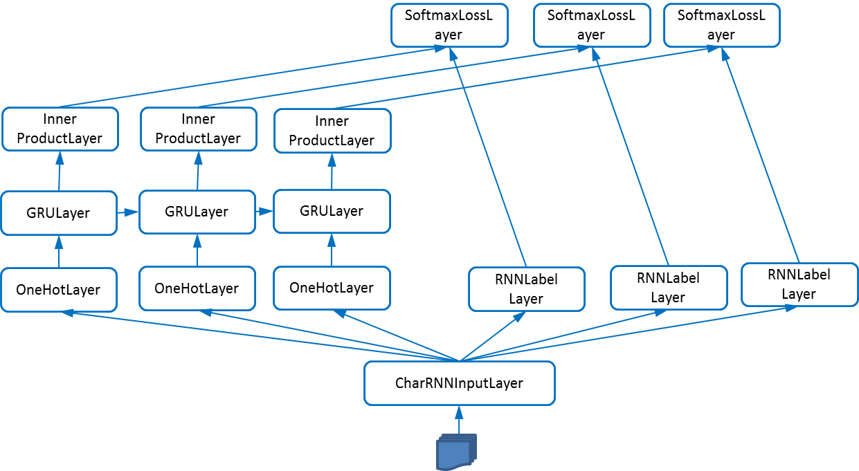
Fig.1 - Illustration of the structure of the Char-RNN model
Fig.1 illustrates the net structure of the char-rnn model. The input layer buffers all training data (the Linux kernel code is about 6MB). For each iteration, it reads unroll_len +1 (unroll_len is configured by users) successive characters, e.g., “int a;”, and passes the first unroll_len characters to OneHotLayers (one per layer). Every OneHotLayer converts its character into the one-hot vector representation. The input layer passes the last unroll_len characters as labels to the RNNLabelLayer (the label of the i-th character is the i+1 character, i.e., the objective is to predict the next character). Each GRULayer receives an one-hot vector and the hidden feature vector from its precedent layer. After some feature transformation, its own feature vector is passed to an inner-product layer and its successive GRULayer. The i-th SoftmaxLossLayer measures the cross-entropy loss for predicting the i-th character. According to Karpathy, there could be another stack of GRULayers connecting the first stack of GRULayers, which improves the performance if there is enough training data. The layer configuration is similar to that for other models, e.g., feed-forward models. The major difference is on the connection configuration.
To model the long dependency, recurrent layers need to be unrolled many times, denoted as unroll_len (i.e., 50). According to our unified neural net representation, the neural net should have configurations for unroll_len recurrent layers. It is tedious to let users configure these layers manually. Hence, SINGA makes it a configuration field for each layer. For example, to unroll the GRULayer, users just configure it as,
layer {
  type: kGRU
  unroll_len: 50
}
Not only the GRULayer is unrolled, other layers like InnerProductLayer and SoftmaxLossLayer, are also unrolled. To simplify the configuration, SINGA provides a unroll_len field in the net configuration, which sets the unroll_len of each layer configuration if the unroll_len is not configured explicitly for that layer. For instance, SINGA would set the unroll_len of the GRULayer to 50 implicitly for the following configuration.
net {
  unroll_len: 50
   layer {
     type: kCharRNNInput
     unroll_len: 1  // configure it explicitly
   }
   layer {
     type: kGRU
     // no configuration for unroll_len
    }
 }
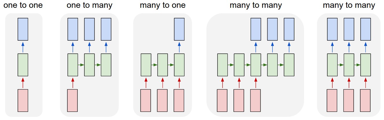
Fig.1 - Different RNN structures from Karpathy
There would be many types of connections between layers in RNN models as shown by Karpathy in Fig.2. For each srclayer, there is a connection_type for it. Taking the i-th srclayer as an example, if its connection type is,
User configured neural net is preprocessed to unroll the recurrent layers, i.e., duplicating the configuration of the GRULayers, renaming the name of each layer with unrolling index, and re-configuring the srclayer field. After preprocessing, each layer’s name is changed to <unrolling_index>#<user_configured_name>. Consequently, the (unrolled) neural net configuration passed to NeuralNet class includes all layers and their connections. The NeuralNet class creates and setup each layer in the same way as for other models. For example, after partitioning, each layer’s name is changed to <layer_name>@<partition_index>. One difference is that it has some special code for sharing Param data and grad Blobs for layers unrolled from the same original layer.
Users can visualize the neural net structure using the Python script tool/graph.py and the files in WORKSPACE/visualization/. For example, after the training program is started,
python tool/graph.py examples/char-rnn/visualization/train_net.json
The generated image file is shown in Fig.3 for unroll_len=5,
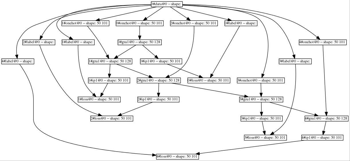
Fig.3 - Net structure generated by SINGA
The BPTT (back-propagation through time) algorithm is typically used to compute gradients of the objective loss w.r.t. parameters for RNN models. It forwards propagates through all unrolled layers (i.e., timepoints) to compute features of each layer, and backwards propagates to compute gradients of parameters. It is the same as the BP algorithm for feed-forward models if the recurrent layers are unrolled infinite times. In practice, due to the constraint of memory, the truncated BPTT is widely used. It unrolls the recurrent layers a fixed (truncated) times (controlled by unroll_len). In SINGA, a BPTTWorker is provided to run the truncated BPTT algorithm for each mini-batch (i.e., iteration). The pseudo code is
BPTTWorker::Forward(phase, net) {
  for each layer in net
    if layer.unroll_index() == 0
      Get(layer.params());   // fetch params values from servers
    srclayers = layer.srclayer();
    if phase & kTest
      srclayers.push_back(net->GetConextLayer(layer))
    layer.ComputeFeature(phase, srclayers)
}

BPTTWorker::Backward(phase, net) {
  for each layer in reverse(net.layers())
    layer.ComputeGradient(layer.srclayers())
    if layer.unroll_index() == 0
      Update(layer.params());   // send params gradients to servers
}
The testing phase is processed specially. Because the test phase may sample a long sequence of data (e.g., sampling a piece of Linux kernel code), which requires many unrolled layers (e.g., more than 1000 characters/layers). But we cannot unroll the recurrent layers too many times due to memory constraint. The special line add the 0-th unrolled layer as one of its own source layer. Consequently, it dynamically adds a recurrent connection to the recurrent layer (e.g., GRULayer). Then we can sample from the model for infinite times. Taking the char-rnn model as an example, the test job can be configured as
test_steps: 10000
train_one_batch {
  Alg: kBPTT
}
net {
  // do not set the unroll_len
  layer {
    // do not set the unroll_len
  }
  …
}
The instructions for running test is the same for feed-forward models.