Canopy Clustering

Canopy Clustering is a very simple, fast and surprisingly accurate method for grouping objects into clusters. All objects are represented as a point in a multidimensional feature space. The algorithm uses a fast approximate distance metric and two distance thresholds T1 > T2 for processing. The basic algorithm is to begin with a set of points and remove one at random. Create a Canopy containing this point and iterate through the remainder of the point set. At each point, if its distance from the first point is < T1, then add the point to the cluster. If, in addition, the distance is < T2, then remove the point from the set. This way points that are very close to the original will avoid all further processing. The algorithm loops until the initial set is empty, accumulating a set of Canopies, each containing one or more points. A given point may occur in more than one Canopy.

Canopy Clustering is often used as an initial step in more rigorous clustering techniques, such as K-Means Clustering . By starting with an initial clustering the number of more expensive distance measurements can be significantly reduced by ignoring points outside of the initial canopies.

WARNING: Canopy is deprecated in the latest release and will be removed once streaming k-means becomes stable enough.

Strategy for parallelization

Looking at the sample Hadoop implementation in http://code.google.com/p/canopy-clustering/ the processing is done in 3 M/R steps:

1. The data is massaged into suitable input format
2. Each mapper performs canopy clustering on the points in its input set and outputs its canopies’ centers
3. The reducer clusters the canopy centers to produce the final canopy centers
4. The points are then clustered into these final canopies

Some ideas can be found in Cluster computing and MapReduce lecture video series [by Google(r)]; Canopy Clustering is discussed in lecture #4 . Finally here is the Wikipedia page .

Design of implementation

The implementation accepts as input Hadoop SequenceFiles containing multidimensional points (VectorWritable). Points may be expressed either as dense or sparse Vectors and processing is done in two phases: Canopy generation and, optionally, Clustering.

Canopy generation phase

During the map step, each mapper processes a subset of the total points and applies the chosen distance measure and thresholds to generate canopies. In the mapper, each point which is found to be within an existing canopy will be added to an internal list of Canopies. After observing all its input vectors, the mapper updates all of its Canopies and normalizes their totals to produce canopy centroids which are output, using a constant key (“centroid”) to a single reducer. The reducer receives all of the initial centroids and again applies the canopy measure and thresholds to produce a final set of canopy centroids which is output (i.e. clustering the cluster centroids). The reducer output format is: SequenceFile(Text, Canopy) with the key encoding the canopy identifier.

Clustering phase

During the clustering phase, each mapper reads the Canopies produced by the first phase. Since all mappers have the same canopy definitions, their outputs will be combined during the shuffle so that each reducer (many are allowed here) will see all of the points assigned to one or more canopies. The output format will then be: SequenceFile(IntWritable, WeightedVectorWritable) with the key encoding the canopyId. The WeightedVectorWritable has two fields: a double weight and a VectorWritable vector. Together they encode the probability that each vector is a member of the given canopy.

Running Canopy Clustering

The canopy clustering algorithm may be run using a command-line invocation on CanopyDriver.main or by making a Java call to CanopyDriver.run(…). Both require several arguments:

Invocation using the command line takes the form:

bin/mahout canopy \
    -i <input vectors directory> \
    -o <output working directory> \
    -dm <DistanceMeasure> \
    -t1 <T1 threshold> \
    -t2 <T2 threshold> \
    -t3 <optional reducer T1 threshold> \
    -t4 <optional reducer T2 threshold> \
    -cf <optional cluster filter size (default: 0)> \
    -ow <overwrite output directory if present>
    -cl <run input vector clustering after computing Canopies>
    -xm <execution method: sequential or mapreduce>

Invocation using Java involves supplying the following arguments:

1. input: a file path string to a directory containing the input data set a SequenceFile(WritableComparable, VectorWritable). The sequence file key is not used.
2. output: a file path string to an empty directory which is used for all output from the algorithm.
3. measure: the fully-qualified class name of an instance of DistanceMeasure which will be used for the clustering.
4. t1: the T1 distance threshold used for clustering.
5. t2: the T2 distance threshold used for clustering.
6. t3: the optional T1 distance threshold used by the reducer for clustering. If not specified, T1 is used by the reducer.
7. t4: the optional T2 distance threshold used by the reducer for clustering. If not specified, T2 is used by the reducer.
8. clusterFilter: the minimum size for canopies to be output by the algorithm. Affects both sequential and mapreduce execution modes, and mapper and reducer outputs.
9. runClustering: a boolean indicating, if true, that the clustering step is to be executed after clusters have been determined.
10. runSequential: a boolean indicating, if true, that the computation is to be run in memory using the reference Canopy implementation. Note: that the sequential implementation performs a single pass through the input vectors whereas the MapReduce implementation performs two passes (once in the mapper and again in the reducer). The MapReduce implementation will typically produce less clusters than the sequential implementation as a result.

After running the algorithm, the output directory will contain:

1. clusters-0: a directory containing SequenceFiles(Text, Canopy) produced by the algorithm. The Text key contains the cluster identifier of the Canopy.
2. clusteredPoints: (if runClustering enabled) a directory containing SequenceFile(IntWritable, WeightedVectorWritable). The IntWritable key is the canopyId. The WeightedVectorWritable value is a bean containing a double weight and a VectorWritable vector where the weight indicates the probability that the vector is a member of the canopy. For canopy clustering, the weights are computed as 1/(1+distance) where the distance is between the cluster center and the vector using the chosen DistanceMeasure.

Examples

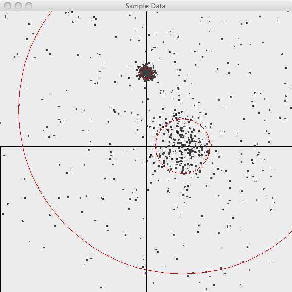
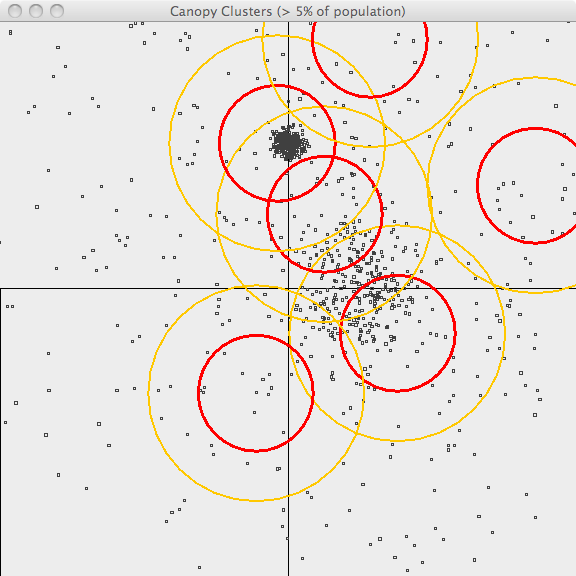
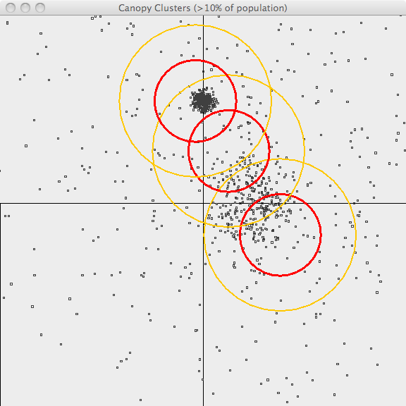
The following images illustrate Canopy clustering applied to a set of randomly-generated 2-d data points. The points are generated using a normal distribution centered at a mean location and with a constant standard deviation. See the README file in the /examples/src/main/java/org/apache/mahout/clustering/display/README.txt for details on running similar examples.

The points are generated as follows:

• 500 samples m=[1.0, 1.0](1.0,-1.0.html) sd=3.0
• 300 samples m=[1.0, 0.0](1.0,-0.0.html) sd=0.5
• 300 samples m=[0.0, 2.0](0.0,-2.0.html) sd=0.1

In the first image, the points are plotted and the 3-sigma boundaries of their generator are superimposed.

In the second image, the resulting canopies are shown superimposed upon the sample data. Each canopy is represented by two circles, with radius T1 and radius T2.

The third image uses the same values of T1 and T2 but only superimposes canopies covering more than 10% of the population. This is a bit better representation of the data but it still has lots of room for improvement. The advantage of Canopy clustering is that it is single-pass and fast enough to iterate runs using different T1, T2 parameters and display thresholds.